초록
X선 광자 상관 분광법(XPCS)은 나노미터 규모의 동역학을 분석할 수 있는 수단을 제공하지만, 그 데이터를 해석하기 위한 실용적인 접근법은 여전히 제한적이다. 본 튜토리얼은 NSLS-II CHX 빔라인에서 수행된 측정을 예시로 들어, XPCS 데이터 분석을 위한 체계적인 프레임워크를 제시한다. 스펙클 패턴과 강도 자기상관계수의 기본 개념을 소개한 뒤, 편극 스위칭과 상전이 동역학이 XPCS 측정에서 어떻게 추출될 수 있는지 보여주는 강유전체 사례 연구를 다룬다. 데이터 해석을 위해 X선 투과율과 같은 탐지된 범위의 실험 조건이 미치는 영향도 검토한다. 이러한 요소들은 XPCS 데이터의 신뢰할 수 있는 분석을 위한 실용적인 지침으로 통합된다.
-
KEYWORDS: X선 광자 상관 분광법(XPCS), 스펙클 패턴, 자기상관계수, 강유전체 도메인 동역학, 상전이
ABSTRACT
X-ray photon correlation spectroscopy (XPCS) provides access to nanoscale dynamics, yet practical approaches for interpreting its data remain limited. This tutorial presents a systematic framework for XPCS data analysis, illustrated using measurements performed at the NSLS-II CHX beamline. The fundamental concepts of speckle pattern and the intensity autocorrelation function are introduced, followed by ferroelectric case studies demonstrating how polarization switching and phase transition dynamics can be extracted from XPCS measurements. The influence of the probed q-range experimental conditions such as X-ray transmittance is examined for data interpretation. These elements are consolidated into practical guidelines for the reliable analysis of XPCS data.
-
KEYWORDS: X-ray photon correlation spectroscopy (XPCS), Speckle pattern, Autocorrelation function, Ferroelectric domain dynamics, Phase transition
1 Introduction
∎ Spectroscopic techniques are widely used to characterize the structure and properties of materials. Conventional X-ray scattering and diffraction, based on interference arising from atomic arrangements, provide average static structural information. However, these methods cannot capture structural changes as they develop over time. Because the measured signals are averaged over time and space, the temporal correlations of microscopic structural fluctuations remain inaccessible.
∎ X-ray photon correlation spectroscopy (XPCS) extends conventional scattering by using coherent X-rays. This makes it possible to track fluctuations in the scattered intensity over time. In this way, XPCS overcomes the time-averaging limitation described above [
1]. The technique can be understood as an X-ray analog of dynamic light scattering (DLS). Conventional DLS uses coherent visible light to track the motion of particles in solution. XPCS instead uses coherent X-rays to generate speckle patterns that reflect the instantaneous internal arrangement of a material. As the internal structure evolves, the resulting changes in the speckle pattern reveal the underlying dynamics.
∎ This tutorial focuses on practical approaches for analyzing and interpreting XPCS data. The measurements were performed at the Coherent Hard X-ray Scattering (CHX) beamline of the National Synchrotron Light Source II (NSLS-II). Ferroelectric Pb(Mg1/3Nb2/3)O3-PbTiO3 (PMN-PT) single crystals are used as a representative example to illustrate how measured speckle patterns can be connected to physical interpretation. The following section introduces the fundamental properties of speckle patterns observed in coherent X-ray scattering.
2 Understanding Speckle Patterns
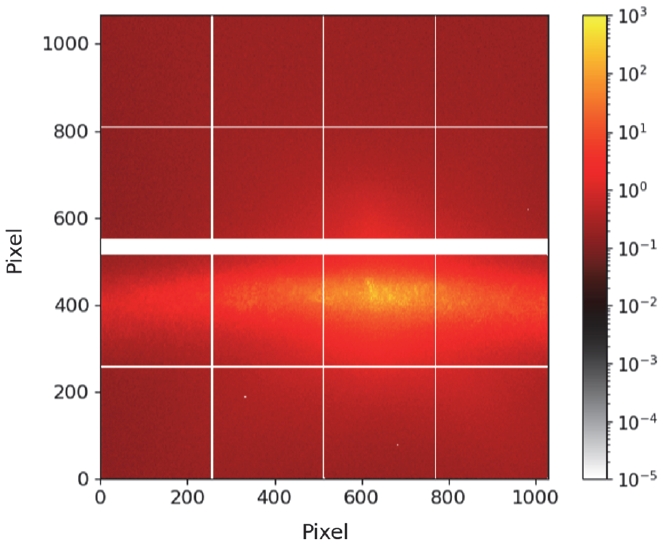
∎ When coherent X-rays illuminate a sample, the scattered X-rays interfere to produce a speckle pattern on the detector (
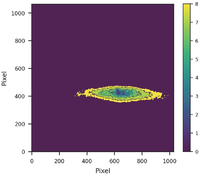
Fig. 1). For crystalline materials, strong scattering peaks appear at specific scattering vectors that satisfy the condition for constructive interference. Even within these peak regions, the illuminated volume is rarely a single uniform lattice. It instead contains nanoscale heterogeneities such as defects, grain boundaries, or local lattice strain, each scattering with a slightly different phase. The interference among these coherently scattered waves produces a non-uniform speckle contrast that encodes the internal arrangement of the sample. The scattered intensity is recorded as pixel array images on a 2D detector, and regions of interest (ROIs) are often defined to improve the signal-to-noise ratio.
Fig. 2 shows an example of an ROI mask in detector pixel space, where the ROIs are ordered from the highest intensity central region outward to the lower intensity regions.
∎ The speckle pattern depends on the phase relationships among the scattered waves. If the sample structure is static, the detector image remains statistically constant over time. When structural changes occur, variations in phase relationships cause the pixel intensity to fluctuate. Each detector pixel corresponds to a scattering vector,
q , determined by the experimental geometry, allowing the speckle intensity to be analyzed in reciprocal space. Different
q ranges probe different length scales. Smaller
q values correspond to larger structural features, whereas larger
q values probe finer details. Temporal changes in the speckle intensity reflect structural evolution at a given
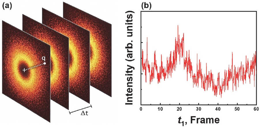
q.
Fig. 3 shows an example of time-dependent speckle data, where these fluctuations form the basis for extracting dynamics through correlation analysis.
3 Dynamics from Time Correlation Functions
∎ XPCS data are analyzed using the time-varying scattered intensity,
I(q, t). The intensity autocorrelation function,
g2(
q, τ), measures the temporal correlation of the scattered intensity at a delay time τ [
2]:
∎ This autocorrelation is related to the intermediate scattering function (ISF), f(q, τ), through the Siegert relation:
where β is the speckle contrast factor determined by beam coher ence and detector resolution. The ISF describes the relaxation of microscopic structural correlations over time. It is commonly modeled using a stretched or compressed exponential form:
∎ Combining
Eqs. (2) and
(3) gives the standard model for fitting XPCS data:
∎ Here,
τ0 is the characteristic relaxation time and
α describes the relaxation behavior. Typically,
α = 1 corresponds to a simple exponential relaxation. Values of
α < 1 represent a distribution of relaxation times, whereas
α > 1 indicates a compressed exponential behavior driven by collective rearrangements [
3].
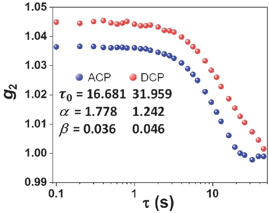
∎ For example,
Fig. 4 compares the XPCS dynamics of PMNPT ferroelectric single crystals under different poling conditions. The decay of
g2(
q, τ) with increasing
τ reflects structural rearrangement. The alternating current poling (ACP) sample exhibits a shorter
τ0 and a larger
α than the direct current poling (DCP) sample, indicating faster relaxation and a compressed exponential motion. In this context, variations between poling conditions can be interpreted in terms of differences in domain structure and stress relaxation. This observation aligns with the larger correlation lengths and domain characteristics reported for ACP samples [
4]. The similar
β values for both samples confirm that the measurements were performed under comparable coherence and detector settings.
∎ The intensity autocorrelation function, g2(q, τ), is obtained by averaging over time. When the dynamics are stationary, the correlation depends only on the time delay τ. However, when the dynamics evolve over time, this averaging can obscure changes in behavior. In such cases, the two-time correlation function is used:
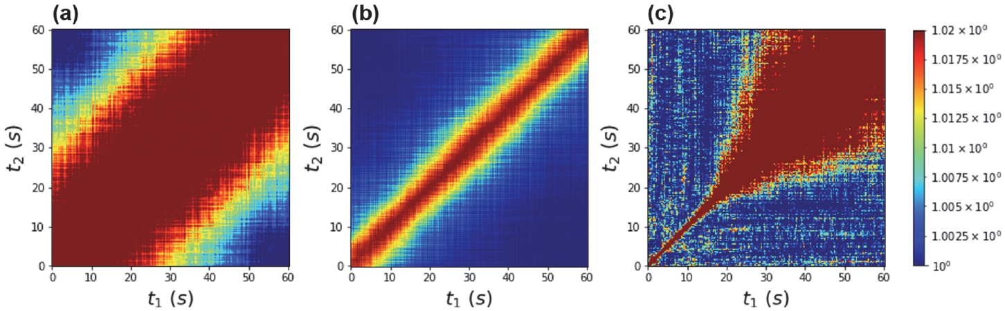
∎ Plotting
C(q, t1, t2) provides a direct visualization of how correlations evolve between two specific times,
t1 and
t2 (
Fig. 5). The diagonal (
t1 =
t2) corresponds to zero delay, and the contour width perpendicular to the diagonal reflects the relaxation time. For stationary dynamics, the correlation remains constant along the diagonal. For non-stationary dynamics, the width changes with time, indicating timedependent relaxation behavior.
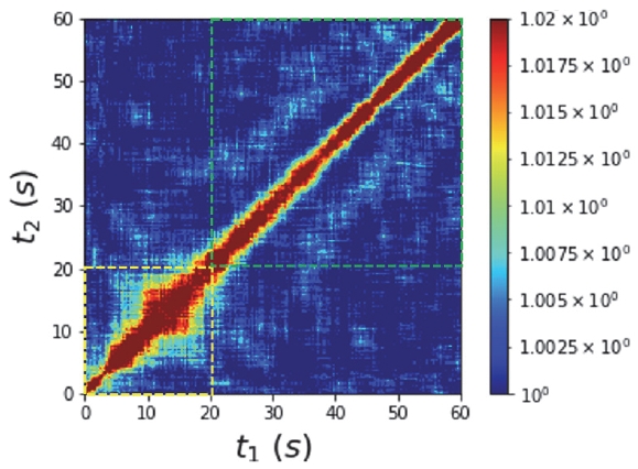
Fig. 6 shows a practical example of heterogeneous dynamics. During the initial stage, the changing contour width indicates non-stationary dynamics. The measurement then transitions to a stationary state characterized by a constant diagonal width. Calculating a single
g2(
q, τ) over the entire measurement obscures changes in the relaxation behavior. In practice, such data are often divided into individual time windows, and
g2(
q, τ) is calculated separately for each segment to track these changes.
4 XPCS Analysis of Ferroelectric Dynamics
∎ Polarization switching in ferroelectrics involves domain wall motion and structural rearrangement occurring over multiple time scales [
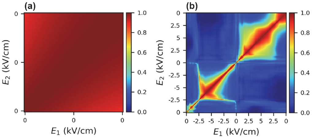
5], which give rise to temporal fluctuations in the speckle pattern. Because the switching process is driven by the applied electric field rather than by time, it is often more informative to analyze the dynamics as a function of field. In this context, the two-time correlation function can be recast into a two-field correlation function, enabling a direct comparison of dynamics at different applied fields (
Fig. 7). The first switching event appears within a relatively narrow field range (−2.5 to −5.0 kV/cm). This confined behavior is likely associated with the several-minute waiting period following the initial poling step, during which defect dipoles can rearrange and establish an internal bias field [
6]. The presence of the internal field can hinder domain wall motion, increasing the coercive field and restricting switching to a limited field range. In contrast, the second switching event extends over a broader field range (0 to +5.0 kV/cm). Since this event follows immediately after the first switching without an intervening waiting period, the domain walls are less influenced by such pinning effects. As a result, switching occurs more gradually across domains, leading to a broader distribution of switching fields. This comparison illustrates how the width of the correlation feature reflects the switching history of the sample, providing insight into whether domain wall motion is constrained or more freely evolving under the applied field.
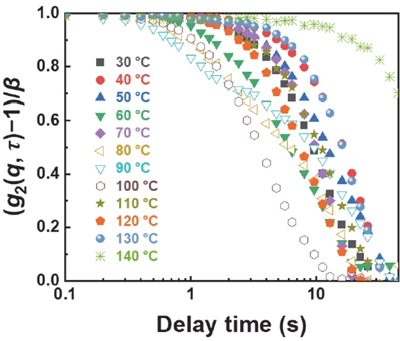
∎ XPCS can also be used to examine how relaxation dynamics depend on temperature.
Fig. 8 shows
g2(
q, τ) measured under isothermal conditions between 30 and 140°C, normalized as (
g2(
q, τ) - 1/
β. This normalization removes differences in the initial speckle contrast (
β), allowing relaxation dynamics at different temperatures to be compared on a common scale. The normalized
g2(
q, τ) curves decay more slowly at longer delay times. Specifically, the relaxation time reaches a minimum between 90°C and 100°C and increases again at higher temperatures, particularly between 130°C and 140°C. For the PMN-PT single crystals used here, temperatures around 90°C and 130°C correspond to the rhombohedraltetragonal phase transition (
TR–T) and the Curie temperature (
TC), respectively [
7]. At
TR–T, the transition between two ferroelectric phases is generally associated with a reduced energy barrier for polarization rearrangement, resulting in faster dynamics. Conversely, the slower relaxation near
TC is consistent with critical slowing down, which is typically attributed to enhanced order-parameter fluctuations as the spontaneous polarization disappears. The temperature dependence of the relaxation time provides a dynamic signature of the phase transitions.
5 Guidelines for Data Interpretation
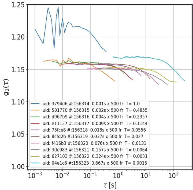
∎ A common pitfall in XPCS analysis is prioritizing results from q regions with a high signal-to-noise ratio (SNR) over those with weaker signals. Low-q regions generally exhibit strong scattering intensities and favorable statistics, whereas high-q correlation curves are often obscured by noise. However, the relaxation behavior observed at low q reflects large-scale structural changes, such as macroscopic domain arrangements, and does not necessarily capture local rearrangements at smaller length scales. In our previous analysis, the temperature dependence of the relaxation time derived solely from low-q data exhibited a different trend than when evaluated across a broader q range. Therefore, a high SNR in a specific q region is generally insufficient to justify using its dynamics as representative of the overall dynamics. In practice, data from multiple q regions are compared to identify the specific length scales associated with the observed structural changes.
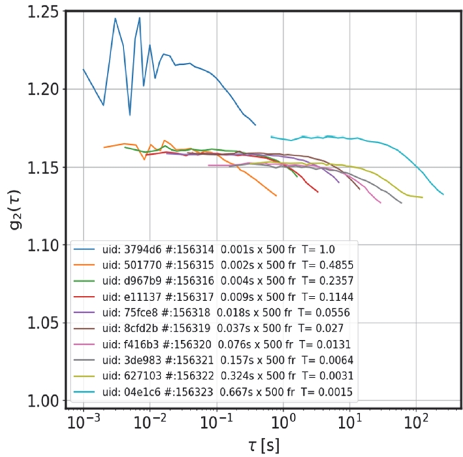
∎ Increasing the X-ray intensity improves the SNR, but excessive flux can distort the data.
Fig. 9 compares the
g2(
τ) curves measured on the same sample at X-ray transmissions ranging from 100% to 0.15%. At 100% transmission, the
g2(
τ) values fluctuate severely at short τ and the baseline is notably elevated compared to other conditions. This anomalous behavior is likely attributed to detector saturation caused by excessive photon flux, combined with poor statistics from the correspondingly short exposure times. At lower transmissions, the overall decay behavior remained similar, although slight differences were observed in the onset of the decay and the slope in the late- region. This indicates that transmission changes within this range do not severely distort the relaxation behavior, though subtle dose-dependent differences may still exist. Additionally, because lower transmission requires longer exposure times to maintain an adequate SNR, the minimum accessible delay time increases. This limits the ability to probe short-time dynamics. Therefore, verifying the absence of non-linear distortions under high-intensity conditions is an essential preliminary step. In practice, the incident X-ray intensity and exposure time are optimized to adequately resolve the time scales of interest without compromising data integrity.
6 Conclusions
∎ This tutorial outlines a practical framework for interpreting XPCS data by linking speckle fluctuations to underlying structural dynamics. The intensity autocorrelation function, g2(q, τ), serves as a primary tool for quantifying relaxation behavior, while complementary correlation analyses capture changes in the dynamics under varying conditions. The examples presented here show that XPCS can resolve structural relaxation across different length scales and external stimuli. The observed dynamics depend on both the probed q-range and the experimental protocol, highlighting the importance of consistent comparison across measurements. From a practical standpoint, careful consideration of measurement conditions is essential. Limited q-ranges may not fully capture the overall dynamics, and parameters such as X-ray transmission and exposure time must be optimized to balance signal quality and temporal resolution while minimizing artifacts. Together, these considerations provide a foundation for the reliable analysis and interpretation of XPCS measurements in complex materials.
Notes
-
Acknowledgement
This research utilized resources at the 11-ID CHX beamline of the National Synchrotron Light Source II, a U.S. Department of Energy (DOE) Office of Science User Facility operated by Brookhaven National Laboratory under Contract No. DESC0012704. This research was also supported by Korea Electrotechnology Research Institute (KERI) Primary research program through the National Research Council of Science & Technology (NST) funded by the Ministry of Science and ICT (MSIT) (No. 26A01015).
-
Conflict of Interest
The author (Wook Jo) currently serves on the editorial board of JEEM, but was not involved in any part of the publication process. Other than this, the authors declare that they have no relevant potential conflicts of interest.
-
Author Contributions
Jeong-Woo Sun: Writing - Original Draft.
Jong Eun Ryu: Funding acquisition, Supervision.
Wook Jo: Writing - Review & Editing, Funding acquisition, Supervision.
Data Availability
Data derived from public domain resources.
Fig. 1.Speckle pattern with intensity distribution in pixel space
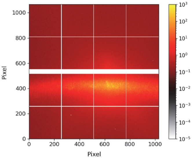
Fig. 2.Example of regions of interest (ROIs) mask obtained by intensity-based segmentation. ROIs are numbered 0–8 in order of decreasing intensity percentile
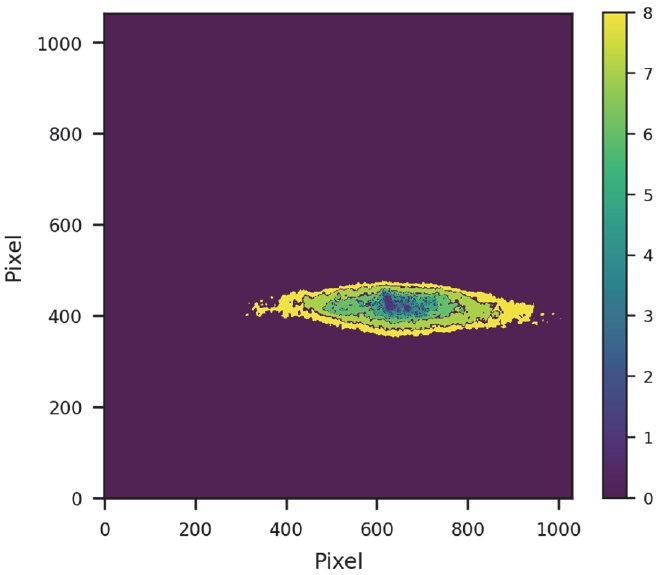
Fig. 3.(a) Speckle patterns at different times with scattering vector q and delay time ∆t. (b) Intensity profile at fixed q as a function of time t1
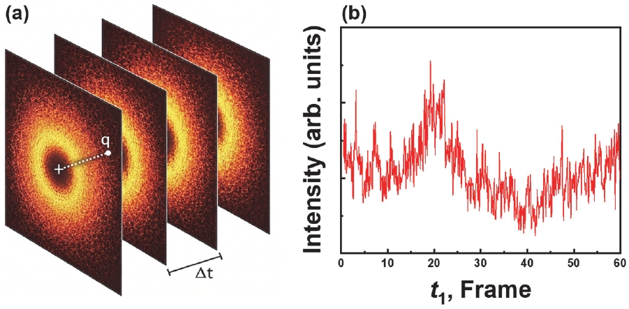
Fig. 4.The intensity autocorrelation function g2(q, τ) for PMNPT ferroelectric single crystals under different poling conditions
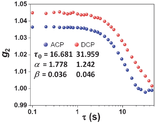
Fig. 5.(a) Two-time correlation map in a stationary state with slow dynamics, showing a broad diagonal feature. (b) Two-time correlation map in a stationary state with fast dynamics, exhibiting a narrow diagonal feature. (c) Two-time correlation map in a non-stationary state with a fanout pattern
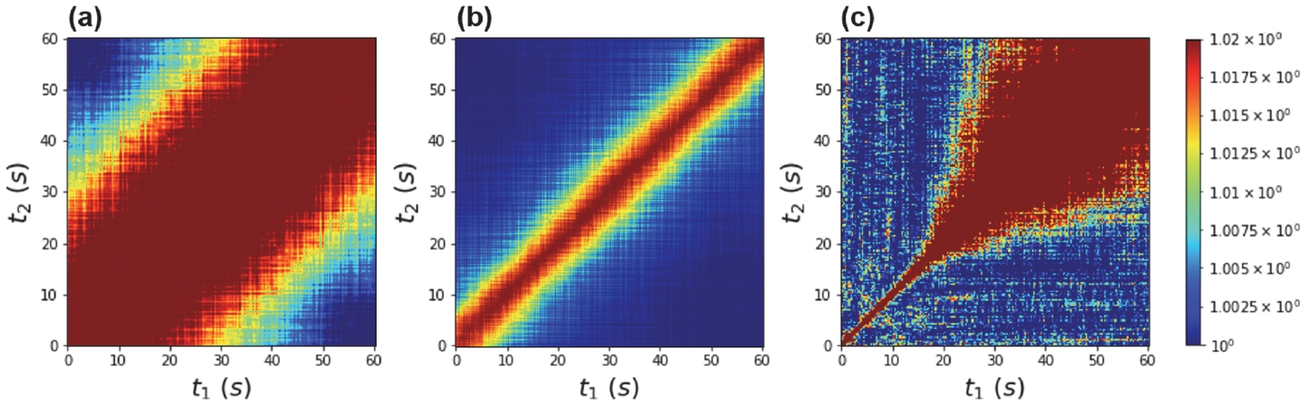
Fig. 6.Two-time correlation map with a non-stationary regime before 20s and a stationary regime at longer times
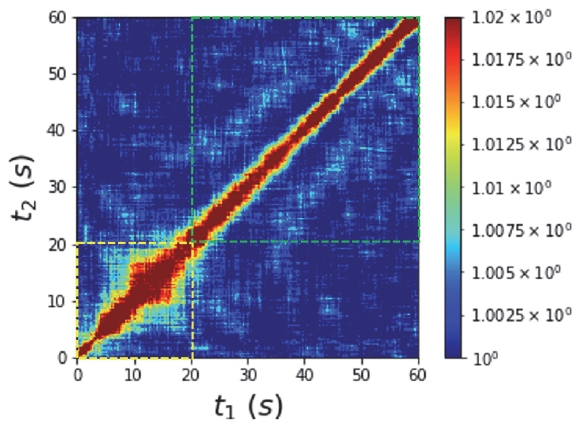
Fig. 7.(a) Two-field correlation map in the absence of an external electric field, showing a stationary state. (b) Two-field correlation function quantifying speckle fluctuations between pairs of electric field values E1 and E2
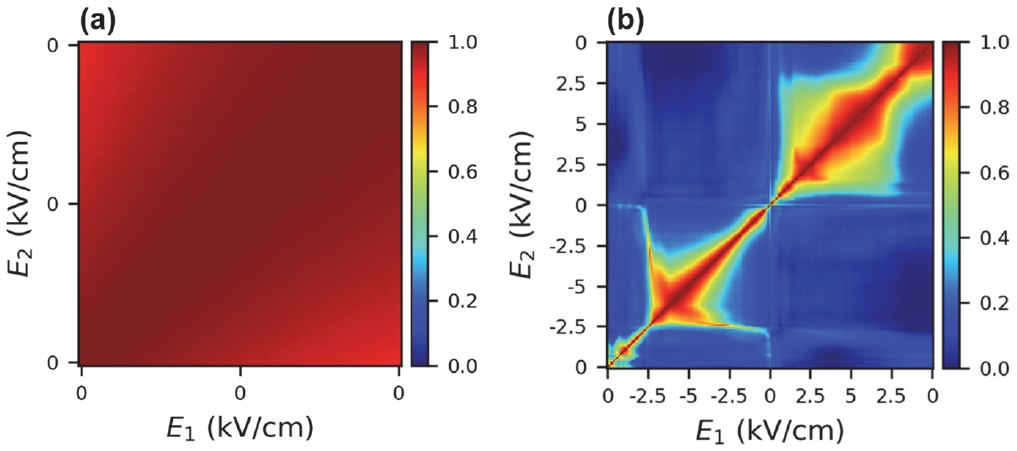
Fig. 8.Normalized intensity autocorrelation functions (g2(q, τ)-1/β as a function of delay time measured at various temperatures during controlled heating
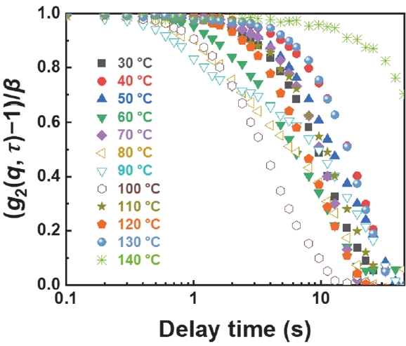
Fig. 9.Intensity autocorrelation functions g2(τ) as a function of delay time for different X-ray transmission levels in a dosedependent study
References
- 1. O. G. Shpyrko, J. Synchrotron Radiat., 21, 1057 (2014). doi: https://doi.org/10.1107/S1600577514018232
- 2. R. L. Leheny, Curr. Opin. Colloid Interface Sci., 17, 3 (2012). doi: https://doi.org/10.1016/j.cocis.2011.11.002
- 3. A. Madsen, A. Fluerasu, and B. Ruta, 2016. Structural Dynamics of Materials Probed by X-Ray Photon Correlation Spectroscopy. In Synchrotron Light Sources and Free-Electron Lasers: Accelerator Physics, Instrumentation and Science Applications, eds. E. J. Jaeschke, S. Khan, J. R. Schneider, and J. B. Hastings. (Springer International Publishing, Cham, Switzerland, 2016), pp. 1617–1641. doi: https://doi.org/10.1007/978-3-319-14394-1_29
- 4. C. Qiu, B. Wang, N. Zhang, S. Zhang, J. Liu, D. Walker, Y. Wang, H. Tian, T. R. Shrout, Z. Xu, L. Q. Chen, and F. Li, Nature, 577, 350 (2020). doi: https://doi.org/10.1038/s41586-019-1891-y
- 5. D. Damjanovic, Rep. Prog. Phys., 61, 1267 (1998). doi: https://doi.org/10.1088/0034-4885/61/9/002
- 6. K. Carl and K. H. Hardtl, Ferroelectrics, 17, 473 (1977). doi: https://doi.org/10.1080/00150197808236770
- 7. S. E. Park and T. R. Shrout, J. Appl. Phys., 82, 1804 (1997). doi: https://doi.org/10.1063/1.365983